Objective
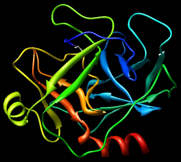
The aim of this tutorial is estimation of protein-ligand binding energy in non-covalent complex between the 1cgh and a small ligand constructed for this purpose.
The second part of this tutorial is Estimation of binding energy using MM-PBSA approach
Stage 1 Editing the pdb file
1) All of the connectivity data at the end of the PDB was removed as this will not be used by XLeap.
2) All protons have been deleted
3) So, residue names of cysteines 42, 58, 136, 168, 182, and 201 have been changed from CYS to CYX.
4) All histidine residues in original 1CGH.pdb file are protonated at both positions, so all HIS residues except for His-57 have been renamed into HIP. His-57 which is a part of a catalytic triad of the enzyme has been renamed into HID
The resulting pdb file is here: 1cgh-modified.pdb
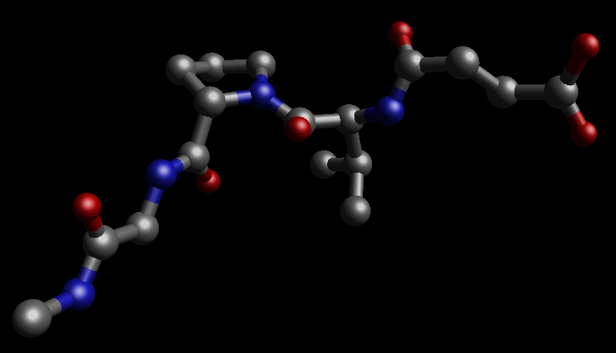
Here is a pdb file of the ligand Sin-Val-Pro-Gly-NMe: ligand.pdb. It was constructed from the original inhibitor Sin-Val-Pro-PPh by substituting the PPh by Gly-NMe.
Stage 2 Create the necessary topology and coordinate files in Xleap
Start Xleap
$AMBERHOME/exe/xleap -s -f $AMBERHOME/dat/leap/cmd/leaprc.ff03
Load library file for SIN residue:
loadoff sin.lib
Load protein and ligand:
protein = loadpdb 1cgh-modified.pdb
ligand = loadpdb ligand.pdb
Add S-S bonds in protein:
bond protein.29.SG protein.45.SG
bond protein.122.SG protein.187.SG
bond protein.152.SG protein.166.SG
Add counter-ions to neutralize a total charge +28 on a protein:
addions protein Cl- 28
Create a complex of a protein and a ligand using combine command:
complex = combine { protein ligand }
Load force field parameters for the SIN residue:
loadamberparams sin.frcmod
Save parameters for sander:
saveamberparm protein protein.top protein.crd
saveamberparm ligand ligand.top ligand.crd
saveamberparm complex complex.top complex.crd
We can save corresponding pdb files for visualization:
savepdb protein protein.pdb
savepdb ligand ligand.pdb
savepdb complex complex.pdb
Stage 3 - Minimise and Equilibrate our Systems
The next stage is to minimize our complex and then use molecular dynamics to sample conformational space. Note, the procedure given here is very short in order to make the simulations compatible with the timescale of this tutorial. In a real "production" simulation you would typically run a much longer simulation (ns) in order to obtain good statistical convergence.
Step 1 let's minimize it to remove any bad contacts created by the hydrogenation and adding counter-ions. In the case of a complex we shall also minimize a fragment of the ligand to remove bad inter-atomic contacts prior to Molecular Dynamics.
Here's our input file, we will do a total of 500 steps of minimisation (MAXCYC) with the first 200 being steepest descent (NCYC), the remainder will be conjugate gradient (MAXCYC-NCYC). We will use a reasonably large cut off of 16 Angstroms since this is not going to be a periodic simulation and we want to deal with our electrostatics accurately (NTB=0,CUT=16). For our implicit solvent model we will use the GB model of Hawkins, Cramer and Truhlar, see the AMBER manual for a full description (IGB=1):
Initial minimisation of our ligand
&cntrl
imin=1, maxcyc=500, ncyc=200,
cut=16, ntb=0, igb=1,
/
Lets run our minimization for the ligand:
$AMBERHOME/exe/sander -O -i ligand-min.in \
-o ligand-min.out \
-p ligand.top \
-c ligand.crd \
For a protein:
Initial minimisation of our protein
&cntrl
imin=1, maxcyc=500, ncyc=200,
cut=16, ntb=0, igb=1,
/
Lets run our minimization for the protein:
$AMBERHOME/exe/sander -O -i protein-min.in \
-o protein-min.out \
-p protein.top \
-c protein.crd \
As for the complex, we shall perform minimization in two steps: the first one will be with the "positional restraints" on each of the protein atoms and on the first three residues of a ligand to keep them essentially fixed in the same position:
complex: initial min of solvent, ions, and part of a ligand
 &cntrl
     imin   = 1,
     maxcyc = 500,
     ncyc   = 250,
     ntb    = 0,
     ntr    = 1,
     cut    = 16,
     igb    = 1
 &end
Hold the protein fixed
100.0
RES 1 224
END
Hold part of a ligand fixed
100.0
RES 330 332
END
END
$AMBERHOME/exe/sander -O -i complex-min.in \
-o complex-min.out -c complex.crd \
-p complex.top -r complex-min.rst \
-ref complex.crd
The second step will be minimization of an entire system:
Minimisation of our complex
 &cntrl
  imin=1, maxcyc=500, ncyc=200,
  cut=16, ntb=0, igb=1,
 /
$AMBERHOME/exe/sander -O -i complex-min2.in \
-o complex-min2.out -c complex-min.rst \
-p complex.top -r complex-min2.rst
You can use ambpdb to generate a pdb of the final minimized structures if you want:
ambpdb -p complex.top <complex-min2.rst > complex_min2.pdb
It is always a good idea to visualize your results and to detect any anomalies.
The next step is to heat and equilibrate our three systems. For speed we will do this very rapidly over 2ps. Ideally, you should do this for much longer.
Then we shall run MD (imin=0) and this is not a restart (irest=0). In this example we will not use shake since it is possible that the hydrogen motion may effect the binding energy (probably not, but it serves as an example here). As we are not using shake we will need a time step smaller than normal. Here we shall use a time step of 1 fs and run for 2000 steps [2 ps] (dt = 0.001, nstlim=2000, ntc=1). We will also write to our output file every 100 steps and to our trajectory [mdcrd] file every 100 steps (ntpr=100, ntwx=100). For temperature control we will use a Langevin dynamics approach with a collision frequency of 1 ps-1. We will start our system at 0K and we want a target temperature of 300K (ntt=3, gamma_ln=1.0, tempi=0.0, temp0=300.0):
Initial MD equilibration
 &cntrl
  imin=0, irest=0,
  nstlim=2000,dt=0.001, ntc=1,
  ntpr=100, ntwx=100,
  cut=16, ntb=0, igb=1,
  ntt=3, gamma_ln=1.0,
  tempi=0.0, temp0=300.0,
 /
We run this 2ps of equilibration for all 3 of our systems (using the final structure from the minimization as our input structure).
$AMBERHOME/exe/sander -O -i initial-md.in \
-o ligand-init-md.out -c ligand-min.rst \
-p ligand.top -r ligand-init-md.rst
$AMBERHOME/exe/sander -O -i initial-md.in \
-o protein-init-md.out -c protein-min.rst \
-p protein.top -r protein-init-md.rst
$AMBERHOME/exe/sander -O -i initial-md.in \
-o complex-init-md.out -c complex-min2.rst \
-p complex.top -r complex-init-md.rst \
Stage 4 - Run Production MD and Estimate the Binding Energy
The final stage now we have equilibrated our system is to run a production simulation. During this time we should monitor the energy of our 3 systems and calculate the average energy over the production run. Fortunately sander does this for us automatically and writes out the average energy at the end of the output file. So, we will run our 3 production calculations. These are identical to the equilibration phase above except that we will state that we are doing a restart so that we read the positions and velocities from the restrt file produced by the equilibration phase. We will also only run our MD for 10ps. Here is the input file:
Production MD
 &cntrl
  imin=0, irest=1, ntx=5,
  nstlim=10000,dt=0.001, ntc=1,
  ntpr=20, ntwx=1000,
  cut=16, ntb=0, igb=1,
  ntt=3, gamma_ln=1.0,
  tempi=300.0, temp0=300.0,
 /
We run this 10 ps of equilibration for all 3 of our systems:
$AMBERHOME/exe/sander -O -i md.in \
-o ligand-md.out -c ligand-init-md.rst \
-p ligand.top -r ligand-md.rst \
-x ligand-md.crd
$AMBERHOME/exe/sander -O -i md.in \
-o protein-md.out -c protein-init-md.rst \
-p protein.top -r protein-md.rst \
-x protein-md.mdcrd
$AMBERHOME/exe/sander -O -i md.in \
-o complex-md.out -c complex-init-md.rst \
-p complex.top -r complex-md.rst \
-x complex-md.crd
We can take a look at the energies in the output files:
For example, for complex:
We can see that we have not equilibrated sufficiently since the mean value of our energy still drifts over time. Thus we cannot expect our calculated binding energy to be accurate. For this tutorial though it will suffice. Now, look at the three output files and find the average energies. The relevant lines are:
Complex:
A V E R A G E S O V E R 10000 S T E P S
 NSTEP =    10000   TIME(PS) =      12.000  TEMP(K) =   294.79  PRESS =     0.0
 Etot   =     -6525.5513  EKtot   =      3425.2364  EPtot      =     -9950.7877
 BOND   =      1414.5269  ANGLE   =      1863.5536  DIHED      =      2074.8398
 1-4 NB =       794.7430  1-4 EEL =      4138.8562  VDWAALS    =     -1813.6935
 EELEC  =    -11382.7410  EGB     =     -7040.8727  RESTRAINT  =         0.0000
 ------------------------------------------------------------------------------
Ligand:
A V E R A G E S O V E R 10000 S T E P S
 NSTEP =    10000   TIME(PS) =      12.000  TEMP(K) =   295.92  PRESS =     0.0
 Etot   =        22.5268  EKtot   =        45.8679  EPtot      =       -23.3411
 BOND   =        18.4360  ANGLE   =        30.1638  DIHED      =        30.9208
 1-4 NB =         9.6937  1-4 EEL =       179.9822  VDWAALS    =        -6.4221
 EELEC  =      -189.6373  EGB     =       -96.4780  RESTRAINT  =         0.0000
 ------------------------------------------------------------------------------
Protein:
A V E R A G E S O V E R 10000 S T E P S
 NSTEP =    10000   TIME(PS) =      12.000  TEMP(K) =   296.53  PRESS =     0.0
 Etot   =     -6462.7596  EKtot   =      3397.6892  EPtot      =     -9860.4488
 BOND   =      1405.8155  ANGLE   =      1845.3059  DIHED      =      2042.4230
 1-4 NB =       785.2541  1-4 EEL =      3950.2549  VDWAALS    =     -1757.6921
 EELEC  =    -11004.4387  EGB     =     -7127.3715  RESTRAINT  =         0.0000
 ------------------------------------------------------------------------------
From these three files we can get the average potential energies of our three systems:
Complex = -9950.79 kcal/mol
Protein = -9860.45 kcal/mol
Peptide = -23.34 kcal/mol
Our binding energy is then simply Ecomplex - Eprotein - Epeptide = -67 kcal/mol
So, our complex is stabilized by about 67 kcal/mol. Note, however, that this value looks too high and that we did not run a long enough equilibration or production run and so our answer is on an approximation at best. Nevertheless you should now be familiar with how to run minimization and molecular dynamics with Amber.
Next Step: Estimation of binding energy using MM-PBSA approach