"Standard" Simulation Setup

Objectives
The purpose of this tutorial is to provide an initial introduction to setting up and running simulations using the AMBER software. In this tutorial we run a series of simulations on a human cathepsin G ? trypsin-like serine proteinase.
We will first figure out how to prepare a starting structure and then use this structure to construct the necessary input files for running sander, the main molecular dynamics engine supplied with AMBER.
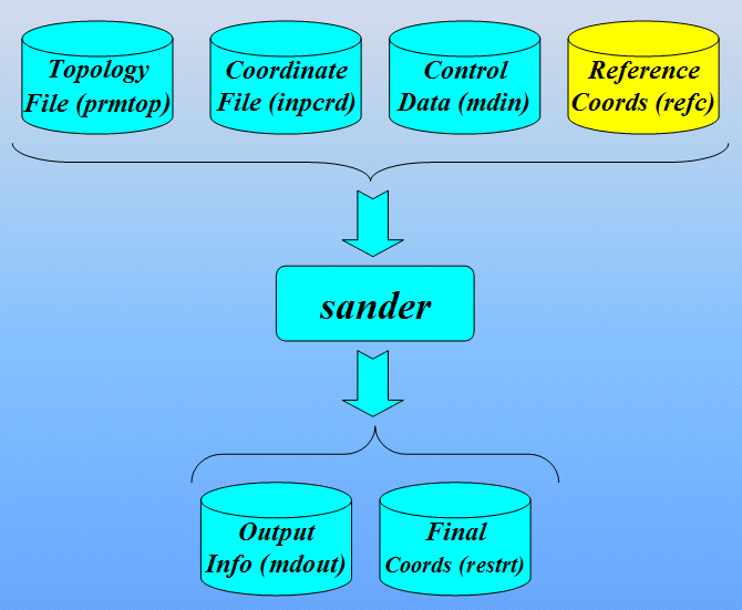
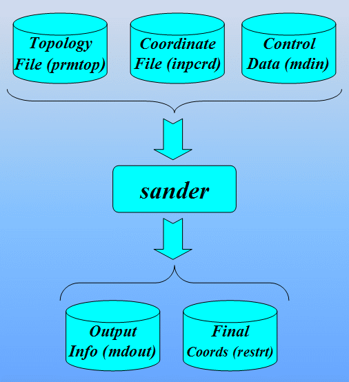
In order to run a classical molecular dynamics simulation with sander a number of files are required. These are (using their default filenames):
- prmtop - a file containing a description of the molecular topology and the necessary force field parameters.
- inpcrd (or a restrt from a previous run) - a file containing a description of the atom coordinates and optionally velocities and current periodic box dimensions.
- mdin - the sander input file consisting of a series of namelists and control variables that determine the options and type of simulation to be run.
First, we shall learn how to edit original pdb file prior to using Amber.
Next, we shall set up the molecular topology/parameter and coordinate files necessary for performing minimization or dynamics using Xleap
Finally, we shall run short MD simulations in-vacuo
Create the necessary topology and coordinate files
The first stage is to create topology (prmtop) and coordinate (inpcrd) files for the system we wish to simulate. We will use Xleap to do this.
The original file, 1CGH.pdb, is an X-ray structure of a human cathepsin G in complex with inhibitor Suc-Val-Pro-Phep-(OPh)2 covalently bonded to the Ser-195 of a protein. For this tutorial we will be using only the protein without inhibitor (and so without non-standard residues).
Editing the pdb file
1) You should always read all of the header information in a pdb file since it often contains important information. For example, in this pdb we see that some waters are too far from the protein:
REMARK 525 SOLVENT
REMARK 525 THE FOLLOWING SOLVENT MOLECULES LIE FARTHER THAN EXPECTED
REMARK 525 FROM THE PROTEIN OR NUCLEIC ACID MOLECULE AND MAY BE
REMARK 525 ASSOCIATED WITH A SYMMETRY RELATED MOLECULE (M=MODEL
REMARK 525 NUMBER; RES=RESIDUE NAME; C=CHAIN IDENTIFIER; SSEQ=SEQUENCE
REMARK 525 NUMBER; I=INSERTION CODE):
REMARK 525
REMARK 525 M RES CSSEQI
REMARK 525 0 HOH 24 DISTANCE = 11.46 ANGSTROMS
REMARK 525 0 HOH 28 DISTANCE = 7.77 ANGSTROMS
REMARK 525 0 HOH 88 DISTANCE = 6.25 ANGSTROMS
REMARK 525 0 HOH 105 DISTANCE = 7.22 ANGSTROMS
REMARK 525 0 HOH 115 DISTANCE = 11.42 ANGSTROMS
In this particular case all water molecules lying more than 3 A from the protein have been deleted.
An inhibitor was also deleted.
2) All of the connectivity data at the end of the PDB was removed as this will not be used by XLeap.
CONECT 286 285 431
CONECT 431 286 430
CONECT 1249 1248 1918
CONECT 1570 1569 1722
3) Some pdb files especially after the NMR refinement contain hydrogen. Converting them from NMR conventions to PDB conventions, experience has shown that hydrogen positions in NMR structures can't always be trusted. Also the naming format for hydrogens could be different from conventions used by xleap. As such a lot of the hydrogen atoms would be seen by xleap to be "extra" atoms for this residue. The best option therefore is to remove all the protons and allow Leap to add them back in at standard positions. Since we will typically minimize our system before running MD this shouldn't pose any problems.
One important point, however, is that having the protons present allows one to check the protonation state of the residues. By default xleap uses the most common protonation states for these residues. For example for histidine a residue name His will by default have epsilon protonation. Thus it is best to go through your protein and ensure that you select the correct protonation state for these residues.
So, all hydrogen atoms from the original pdb file have been deleted.
4) Since pdb files do not distinguish between cysteine residues that are involved in bonds or other things (and hence which have no proton on the sulphur atom) we need to edit the relevant cysteine residues to correct for this. The residue name used by Leap for regular protonated cysteine residues is CYS, for deprotonated (-1 charge) and/or bound to metal atoms it is CYM and for cysteine residues involved in disulphide bridges and other bonds it is CYX.
A header of our pdb file contains information about cysteine residues involved in disulphide bridges:
SSBOND 1 CYS A 42 CYS A 58
SSBOND 2 CYS A 136 CYS A 201
SSBOND 3 CYS A 168 CYS A 182
So, residue names of cysteines 42, 58, 136, 168, 182, and 201 have been changed from CYS to CYX.
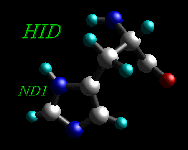
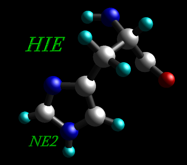
5) Histidine residues can be protonated in the δ ("delta") position (HID), the ε ("epsilon") position (HIE) or at both (HIP).
|
|
Histidine residue protonated in the δ ("delta") position (HID) |
|
|
Histidine residue protonated in the ε ("epsilon") position (HIE) |
|
|
Histidine residue protonated at both positions (HIP) |
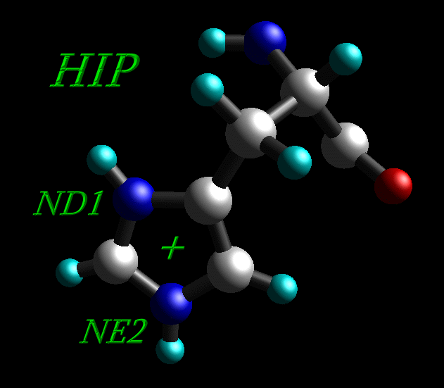
All histidine residues in original 1CGH.pdb file are protonated at both positions, so all HIS residues have been renamed into HIP.
In general case, however, you should go through and carefully check the protonation state of your residues matches what you expect.
6) Some X-ray cannot resolve well Nitrogen and Oxygen atoms in asparagines (ASN) and glutamines (GLN), so these residues should be checked. No changes to the ASN and GLN were made for our structure.
7) Some X-ray structures have more than one conformation for the same residues ("alternate" configurations). By default Leap will use the A conformation and disregard the others.
8) One needs to ensure that there are a TER card between the different chains protein. Otherwise xleap will assume that these are part of the same chain. Our enzyme consists of only one polypeptide chain, however we need to ensure that there is a TER card between the end of a polypeptide chain and water molecules:
ATOM 1784 O SER 224 30.462 27.503 25.760 1.00 0.00
ATOM 1785 CB SER 224 32.731 29.752 24.434 1.00 0.00
ATOM 1786 OG SER 224 31.915 30.536 23.579 1.00 0.00
TER 1786 SER 224
HETATM 1787 O HOH 225 30.319 32.116 2.700 1.00 0.00
HETATM 1788 O HOH 226 10.534 15.138 18.609 1.00 0.00
The final modified pdb file after editing is here: 1cgh-no-inhib.pdb
Loading the structure into Leap
The next step is to use xleap (or tleap) to create the input files for our simulations.
The first step is to start up the graphical version of LEaP:
$AMBERHOME/exe/xleap -s -f $AMBERHOME/dat/leap/cmd/leaprc.ff03
This should load xleap and you should see something like this appear:
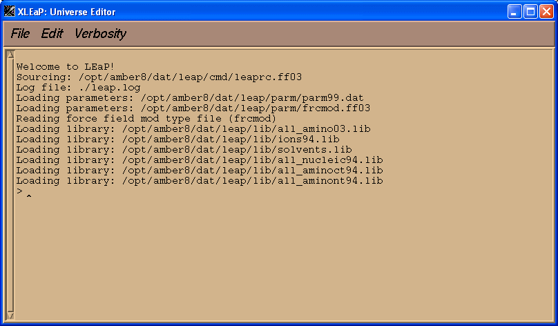
When xleap loads it initially has to open a series of library and parameter files that define the force field parameters to be used and the residue maps etc. Since AMBER 8 (and 9) ships with a range of different force fields, each suited to different types of simulation, it is important to tell xleap which force field we wish to use. This is what the command line options used above are for. The "-s" switch tells xleap to ignore any user defined defaults which might otherwise override our selection, while the "-f $AMBERHOME/dat/leap/cmd/leaprc.ff03" switch tells xleap to execute the start-up script for the FF03 force field. This script contains commands that cause xleap to load all of the configuration files required for the AMBER FF03 force field. If you look in the $AMBERHOME/dat/leap/cmd/ directory you will find a number of different leaprc files such as leaprc.ff03 (FF03 force field), leaprc.ff02ep (FF02 polarisable force field with lone pairs) etc.
To load a pdb into xleap we can use the loadpdb command. This will create a new unit in xleap and load the specified pdb into that unit.
So, to load the pdb file we just created into a new unit called "1cgh" type the following in the xleap window (make sure the xleap window is highlighted and your mouse cursor is within the window):
1cgh=loadpdb 1cgh-no-inhib.pdb
This should result in output, similar to the following, appearing in the xleap window:
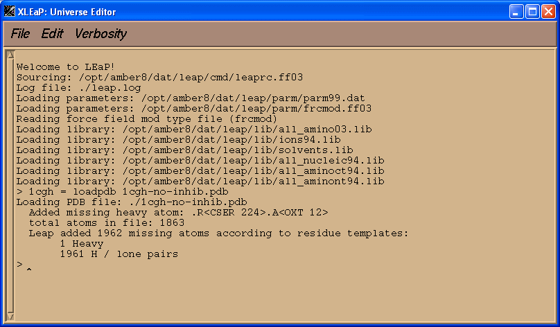
Xleap automatically added all missing hydrogens to all residues as well as a missing Oxygen atom to the C-terminal residue, Ser-224.
To see the structure, in xleap, use the edit command and specify the unit you wish to edit, in this case the one we just created "1cgh":
edit 1cgh
This should open the xleap editor window and display something similar to the following:
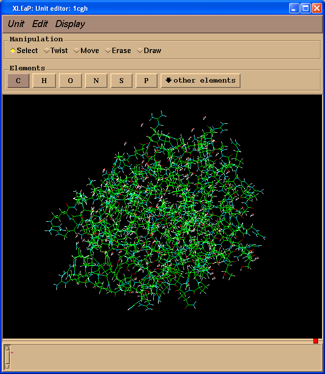
Within this window the LEFT mouse button allows atom selection (drag and drop), the MIDDLE mouse button rotates the molecule and the RIGHT mouse button translates it. If the MIDDLE button does not work you can simulate it by holding down the Ctrl key and the LEFT mouse button. To make the image larger or smaller, simultaneously hold down the MIDDLE and RIGHT buttons (or Ctrl and RIGHT) and move the mouse up to zoom in or down to zoom out.
If you played with selecting atoms using the left mouse button you can unselect a region by holding down the shift key while drawing the selection rectangle. To select everything, double click the LEFT button (and to unselect, do the same while holding down the shift key).
It is always a good idea to look at the models before trying to use them. In this way problems can often be identified before running expensive calculations.
We can check our model using check command
check 1cgh
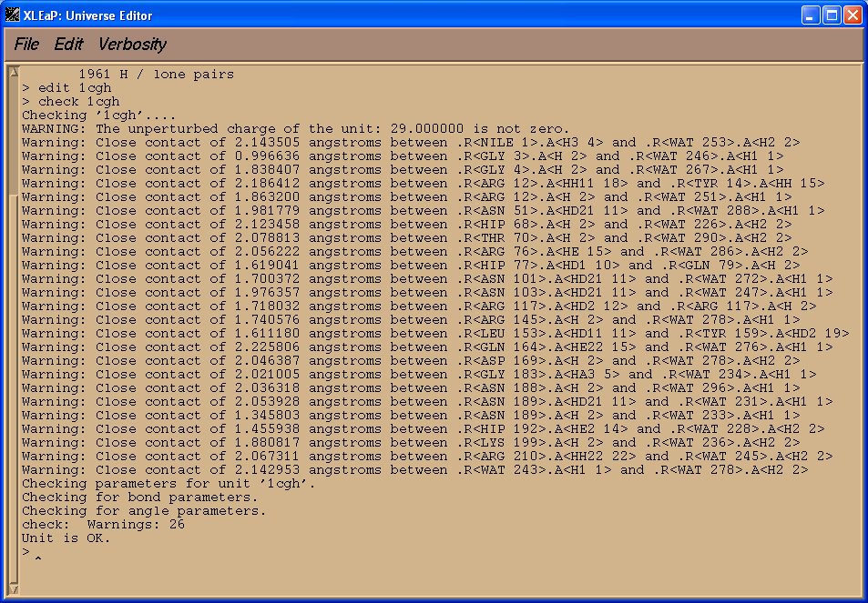
We see that there are many close contacts, mainly between protein residues and water molecules. We see also that a total charge of our molecule is +29 (we shall handle it later).
Now before we go any further we have to ensure that all the bonds between cysteine residues involved in disulphide bridges are defined. At the moment none of the bonds are defined.
Now our residues have different sequence numbers than in original pdp file. We need to add bonds between the sulphur atoms of cysteines 29 and 45, 122 and 187, and 152 and 166. We can do this with the bond command, alternatively we could edit 1cgh and draw in the bond manually but for a protein this is pretty tedious.
> bond 1cgh.29.SG 1cgh.45.SG
> bond 1cgh.122.SG 1cgh.187.SG
> bond 1cgh.152.SG 1cgh.166.SG
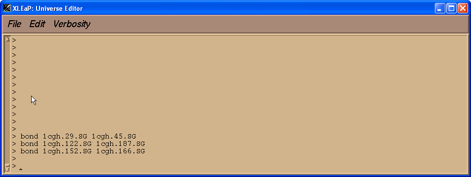
This will create the three missing bonds.
We can save structure created by xleap in the pdb file using command savepdb to be viewed later with a more sophisticated viewing program available
savepdb 1cgh 1cgh-no-inhib-final.pdb
We also save our structure in the Object File Format (off) or library file, so that we don't have to repeat all of the steps we did above. We can just reload the library file:
saveoff 1cgh 1cgh-no-inhib.lib

Here is library file 1cgh-no-inhib.lib
The next thing we need to do is to add counter ions. Before we issue the "addions" command, we need to figure out whether our system is positively charged or negatively charge.? If it is positively charge, we will want to add negatively charged Cl- ions to counter it and if it is negatively charged, then we'll add Na+ to counter it. To calculate the charge of our system, we can use the command "charge" or ?check? (see above):
charge 1cgh
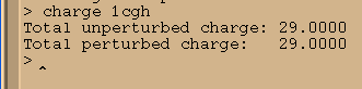
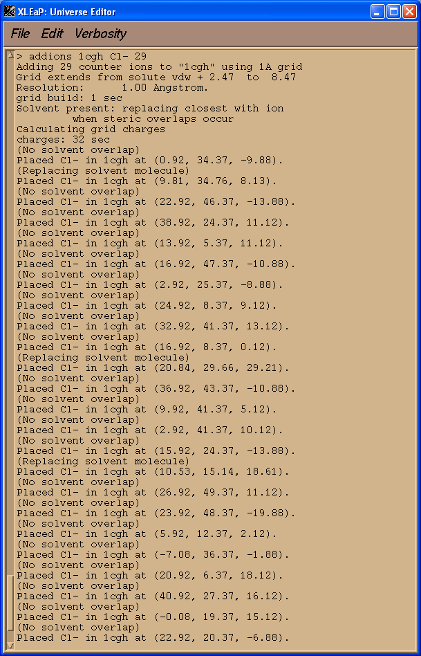
Next we charge neutralise our system since it currently has a charge of +29 (check 1cgh). We shall therefore add a total of 29 Cl- ions.
> addions 1cgh Cl- 29
Saving parameters:
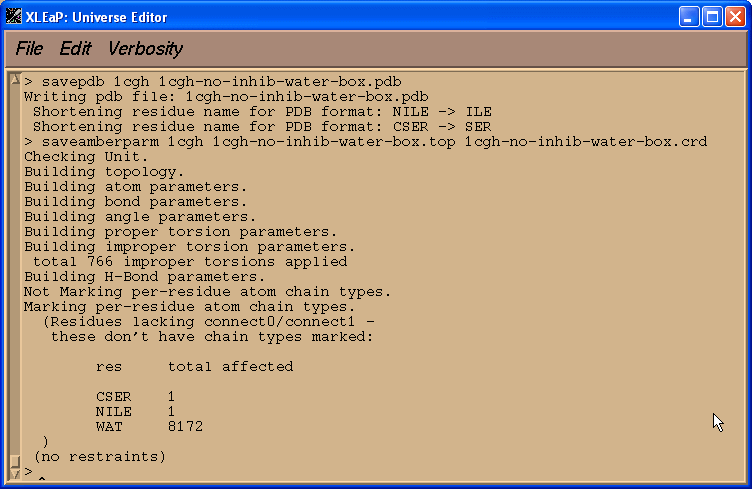
saveamberparm 1cgh 1cgh-no-inhib.top 1cgh-no-inhib.crd
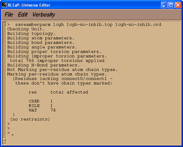
The resulting topology file, 1cgh-no-inhib.top, and file with coordinates 1cgh-no-inhib.crd are quite large.
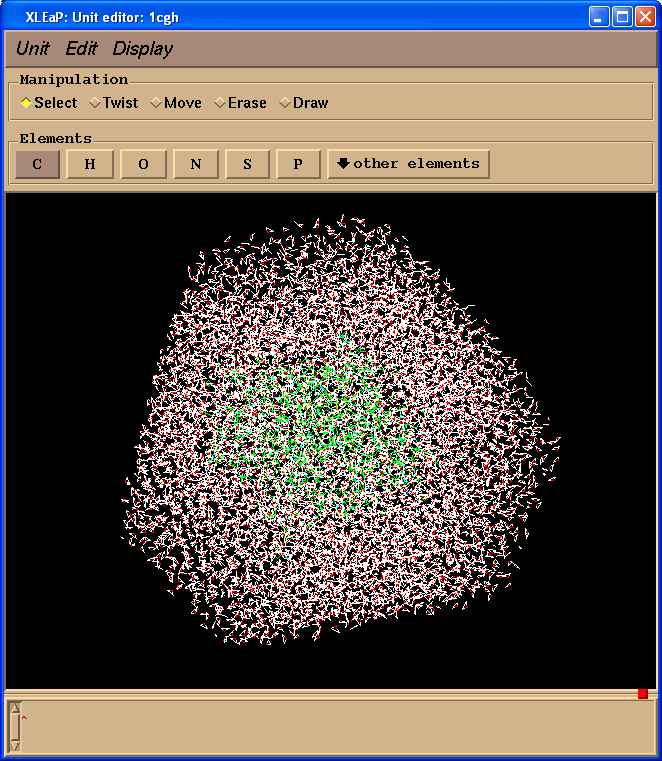
Now we solvate our system in a truncated octahedral box of TIP3P water.
solvateoct 1cgh TIP3PBOX 10
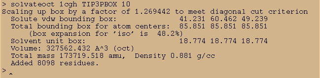
This will add a 10 angstrom buffer of water around our system in addition to the already defined crystallographic waters.
We can save the resulted structure in the pdb file to be viewed later with a more sophisticated viewing program available
savepdb 1cgh 1cgh-no-inhib-water-box.pdb
Saving parameters:
saveamberparm 1cgh 1cgh-no-inhib-water-box.top 1cgh-no-inhib-water-box.crd
edit 1cgh
Preparation of Control Input for Sander
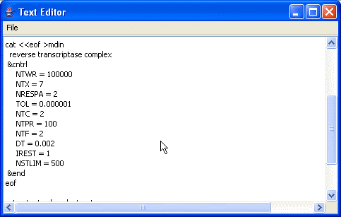
Sample input for Sander, just to establish a basic syntax and appearance.
Minimization with Cartesian restraints
&cntrl
imin=1, maxcyc=200, (invoke minimization)
ntpr=5, (print frequency)
ntr=1, (turn on Cartesian restraints)
restraint_wt=1.0, (force constant for restraint)
restraintmask=?:1-58, (atoms in residues 1-58 restrained)
/
Each of the variables listed aboveis input in a namelist statement with the namelist identifier &cntrl. You can enter the parameters in any order, using keyword identifiers. Variables that are not given in the namelist input retain their default values.
In general, namelist input consists of an arbitrary number of comment cards, followed by a record whose first 7 characters after a " &" (e.g. " &cntrl ") name a group of variables that can be set by name. This is followed by statements of the form " maxcyc=500, diel=2.0, ... ", and is concluded by an " / " token. The first line of input contains a title, which is then followed by the &cntrl namelist. Note that the first character on each line of a namelist block must be a blank.
A Java program has been written at the ANU Supercompuer Center to facilitate preparation of input job control files for Sander-8. It uses intuitive controls to setup job control variables for Sander run. In many cases instead of variable's name it uses variable's description. For example, for variable NSTLIM it uses "Number of MD Steps (nstlim)".
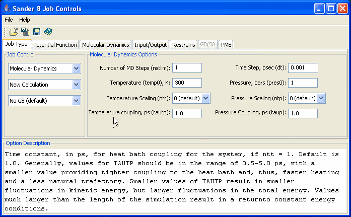
The program has an Option Description panel where it shows a description for every variable each time the user points the cursor onto the variable name/description.
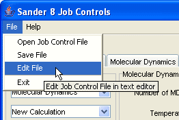
The toolbar provides quick access to commonly used features: Open Sander Job Control file, Reset the variables to their default values, Save Job Control file, and Help
Closely related options are grouped on separated panels which can be activated using tabs.
Options can be setup using either text fields or combo boxes.
Advanced users might want to edit program options using the built-in text editor, with the program allowing easy switching between GUI and text editing.
Currently the program is distributed as a Java JAR file and a set of native executables for some platforms (MS Windows, Mac OS, Linux). To start to use it:
- To run it issue the command "java -jar Sander9Input.jar" in command prompt or double click on it (MS Windows, Mac OS)
- For native executables just type its name in command line or double click on it (MS Windows, Mac OS)
Running Minimisation and MD (in implicit solvent)
This section will introduce sander and show how it can be used for minimization and molecular dynamics of our previously created model. We shall run our simulations with the implicit solvent. For this section of the tutorial we shall be using the in vacuo prmtop and inpcrd files (1cgh-no-inhib.top and 1cgh-no-inhib.crd, correspondingly) we created previously.
Minimisation Stage 1 - Holding the counterions fixed
Our minimization procedure will consist of a two stage approach. In the first stage we will keep the protein fixed and just minimize the positions of the counter-ions and water molecules. Then in the second stage we will minimize the entire system.
There are two options for keeping the protein atoms fixed during the initial minimization.
One method is to use the "BELLY" option in which all the selected atoms have the forces on them zeroed at each step. This results in what is essentially a partial minimization. This method used to be the favoured method but it can, especially if used with constant pressure periodic boundary simulations, lead to instabilities and strange artefacts. As a result of this it is no longer the suggested method.
Instead we shall use "positional restraints" on each of the protein atoms to keep them essentially fixed in the same position. Such restraints work by specifying a reference structure, in this case our starting structure, and then restraining the selected atoms to conform to this structure via the use of a force constant. This can be visualized as basically attaching a spring to each of the solute atoms that connects it to its initial position. Moving the atom from this position results in a force which acts to restore it to the initial position. By varying the magnitude of the force constant so the effect can be increased or decreased. This can be especially useful with structures based on homology models which may be a long way from equilibrium and so require a number of stages of minimization / MD with the force constant being reduced each time.
Here is the input file we shall use for our initial minimization of solvent and ions:
Anions minimization
&cntrl
IGB=5,
CUT=10,
NTR = 1,
NTMIN = 0,
MAXCYC = 500,
NTPR = 100,
NTB=0,
IMIN = 1
&end
Group input for restrained atoms
100.0
RES 1 239
END
END
The meaning of each of the terms are as follows:
- IMIN = 1: Minimisation is turned on (no MD)
- MAXCYC = 500: Conduct a total of 500 steps of minimization.
- NTB = 0: Do not use periodic boundaries
- NTMIN = 0: Use full conjugate gradient minimization.
- CUT = 10: Use a cutoff of 10 angstroms.
- NTR = 1: Use position restraints based on the GROUP input given in the input file. GROUP input is described in detail in the appendix of the user's manual. In this example, we use a force constant of 100 kcal mol-1 angstrom-2 and restrain residues 1 through 239 (the protein). This means that the water and counter-ions are free to move. The GROUP input is the last 5 lines of the input file:
Group input for
restrained atoms
100.0
RES 1 239
END
END
Note that whenever you run using the GROUP option in the input you should carefully check the top of the output file to make sure you've selected as many atoms as you thought you did.
Command to run sander:
$AMBERHOME/exe/sander -O -i 1cgh-no-inhib-fixed-protein.in \
-o 1cgh-no-inhib-fixed-protein.out -c 1cgh-no-inhib.crd \
-p 1cgh-no-inhib.top -r 1cgh-no-fixed-protein.rst \
-ref 1cgh-no-inhib.crd
Input files: 1cgh-no-inhib-fixed-protein.in, 1cgh-no-inhib.crd, 1cgh-no-inhib.top
Output Files: 1cgh-no-inhib-fixed-protein.out, 1cgh-no-fixed-protein.rst
Take a look at the output file from this job. You should notice that there is initially a rather high van-der-Waals (VDWAALS and 1-4 VDW) energy which represents bad contacts in both the water and protein. You should also see that the electrostatic energy (EEL) drops very rapidly. The RESTRAINT energy represents the effect of the harmonic restraints we have imposed. It rises rapidly but then levels off.
Lets take a quick look at the structure, in order to ensure it still sensible, before proceeding:
ambpdb -p 1cgh-no-inhib.top < 1cgh-no-fixed-protein.rst > 1cgh-no-inhib-fixed-protein.pdb

Minimisation Stage 2 - Minimising the entire system
Now we have minimized the water and ions the next stage of our minimization is to minimize the entire system. In this case we will run 500 steps of minimization without the restraints this time. Here is the input file:
Entire system minimization
&cntrl
IGB=5,
CUT=10,
NTMIN = 0,
MAXCYC = 500,
NTPR = 100,
NTB=0,
IMIN = 1
&end
Note, choosing the number of minimization steps to run is a bit of a black art. Running too few can lead to instabilities when you start running MD. Running too many will not do any real harm since we will just get ever closer to the nearest local minima. It will, however, waste cpu time. Since minimization is generally very quick with respect to the molecular dynamics it is often a good idea to run more minimization steps than really necessary. Here, 500 should be enough.
We run this using the following command. Note, we use the 1cgh-no-fixed-protein.rst file from the previous run, which contains the last structure from the first stage of minimization, as the input structure for stage 2 of our minimization. Note, we also no longer need the -ref switch:
$AMBERHOME/exe/sander -O -i 1cgh-no-inhib-all-minimize.in \
-o 1cgh-no-inhib-all-minimize.out -c 1cgh-no-fixed-protein.rst \
-p 1cgh-no-inhib.top -r 1cgh-no-all-minimize.rst
Running MD on the whole system
Now we can run MD simulation for 20 ps.
Here is the input file:
MD run
&cntrl
IGB=5,
CUT=16,
NTMIN = 0,
MAXCYC = 500,
NTPR = 100,
NTB=0,
imin = 0, irest = 0,
ntt=3, gamma_ln=1.0,
tempi=0.0, temp0=300.0,
nstlim=10000,dt=0.002, ntc=2,
ntpr=50, ntwx=500
&end
i.e. we shall run MD (imin=0) and this is not a restart (irest=0). In this example we will use SHAKE (ntc=2). Here we shall use a time step of 2 fs and run for 10000 steps [2 ps] (dt = 0.002, nstlim=10000). We will also write to our output file every 50 steps and to our trajectory [mdcrd] file every 500 steps (ntpr=50, ntwx=500). For temperature control we will use a Langevin dynamics approach with a collision frequency of 1 ps-1. We will start our system at 0K and we want a target temperature of 300K (ntt=3, gamma_ln=1.0, tempi=0.0, temp0=300.0).
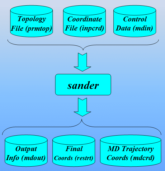
$AMBERHOME/exe/sander -O -i md.in \
-o 1cgh-no-inhib-md.out -c 1cgh-no-all-minimize.rst \
-p 1cgh-no-inhib.top -r 1cgh-md.rst \
Visualizing the trajectories with Chimera
Start Chimera
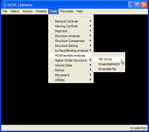
To load a structure select MD Movie from the Tools menu Tools->MD/Ensemble Analysis->MD Movie
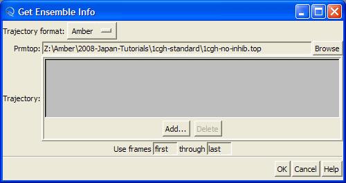
this will open "Get Ensemble Info" dialog
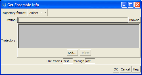
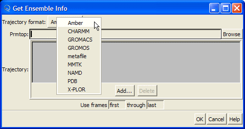
Be sure that "Amber" is selected in the "Trajectory format" combo-box:
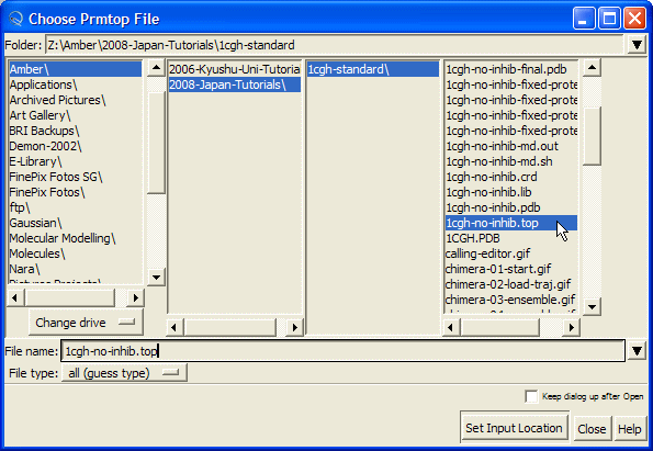
Hit "Browse" button and this will open the "Choose Prmtop File" dialog. Select "1cgh-no-inhib.top" file
Then press "Add" button to load MD trajectory
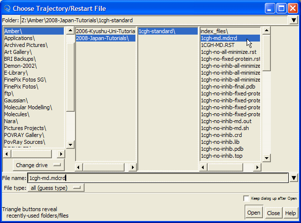
and select "1cgh-md.mdcrd" file and press "Open" button
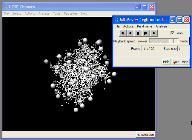
Finally, press "OK" button

Now our molecule is shown in the Main Window. We can now use the playback tools in the "MD Movie: ..." control panel to play our movie
All manipulations with molecular structures are accomplished by pressing mouse button and then moving the mouse. It is strongly advisable to use a three button mouse.
Rotation
Hold down the left mouse button and then move the mouse
Translation
Hold down the middle mouse button and then move the mouse
Scaling (Zooming)
Hold down the right mouse button and then move the mouse
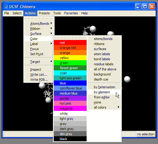
We might want to change atom's colors
Visualizing the trajectories with VMD
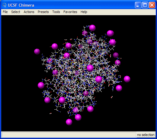
You should have a go at playing the video of the trajectory. Notice how the protein holds its structure there is considerable movement in the extremities but the overall structure is preserved. However, water molecules and some counter-ions flee away from the protein.
The take home lesson here is that you should think very carefully about what you are simulating, Are you really simulating realistic conditions, how are the parameters you have chosen biasing your results? Where does your system evolve to during the MD simulation? A cutoff can be a good way to increase the speed of a simulation, but you need to be aware that it can introduce very large artefacts into your simulation. So, think very carefully, and try out several scenarios before you try to reach firm conclusions.
One way to improve considerably on our in vacuo simulations is to make our physical model of a protein much closer to reality, i.e. include solvent effects via the use of explicit solvent and to use periodic boundary conditions.
If you still want to stick to in vacuo simulations and to use the implicit solvation models you might want to try a following scenario: delete water molecule which fled away from the protein and add constraints to keep counter-ions near the corresponding charged residues.