
Though Gaussian has necessary facilities for finding the exact stationary points (either equilibrium structures or Saddle Points of the nth order), locating the Transition States is usually more tricky task than a simple geometry minimization. So, prior to applying the exact methods for finding the Transition State it is a good idea to perform the Potential Energy Scan (PES) to explore a region of a potential energy surface. To request a PES in Gaussian one needs to specify the reaction variable(s) and their range for scan. Molecular structure at each point of the scan can be either kept rigid (a rigid PES scan which consists of single point energy evaluations) or be optimized (a relaxed PES scan with geometry optimization at each point which is requested with the Opt keyword).
![]() It's advisable to start PES using the inexpensive computational methods, for example, HF/3-21G to get quickly the overall picture of the Potential Energy Surface along the reaction coordinate(s).
It's advisable to start PES using the inexpensive computational methods, for example, HF/3-21G to get quickly the overall picture of the Potential Energy Surface along the reaction coordinate(s).
We shall study a double bond migration in CH3CHCH2:

and perform a PES of a Hydrogen atom migration from one Carbon atom to another, so we shall define a distance between a Hydrogen and distant Carbon atom as a reaction coordinate:
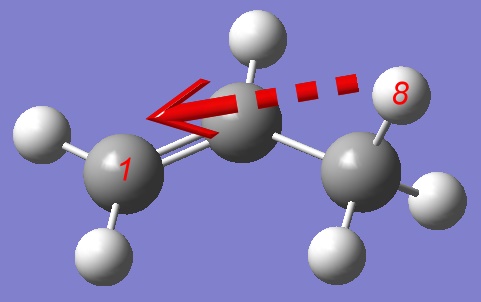
The resulting Gaussian input is below:
# opt=modredundant hf/3-21g Hydrogen atom migration PES 0 1 C -1.27051500 -0.22247300 -0.00000200 H -2.22577000 0.26685300 -0.00000200 H -1.28510700 -1.29696200 -0.00001100 C -0.14350900 0.45672400 0.00001600 H -0.17197800 1.53256300 -0.00005500 C 1.23364500 -0.16153700 0.00000100 H 1.17645900 -1.24331300 -0.00041900 H 1.79448100 0.15260400 -0.87526600 H 1.79418500 0.15196900 0.87566100 B 1 8 S 21 -0.100000 |
Modreduntant option tells Gaussian to modify coordinate definition before performing the calculation and it requires a separate input section following the geometry specification.
B 1 8 S 21 -0.100000 is a Modreduntant section where "B" means a bond length defined by atoms "1" and "8". "S" tells Gaussian to perform a relaxed Potential Energy Surface Scan incrementing the coordinate by a stepsize "-0.100000" a total of nsteps "21" times, performing an optimization from each resulting starting geometry. Numbers "-0.100000" and "21" are used because of the initial 3.21 Å distance between the Hydrogen and Carbon atoms (you can check it in your favorite molecular editor), so a PES scan is supposed to run for a C-H distance from 3.21 to 1.11 Å with a -0.1 increment (or 0.1 decrement).
We can visualize the results of the PES in GaussView:
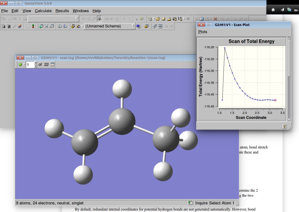
A plot of the Potential Energy Surface Scan shows that we have a saddle point. A plot is interactive, so you can click on the various points in the plot, and the corresponding structure will appear in the Molecular View window. We shall select a structure corresponding to the highest Total Energy (Saddle Point):
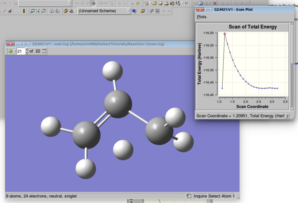
By pressing the green circle button in the toolbar of the Molecular View window you can animate the various structures. The animation can then be stopped via the red X icon which replaces it.
So, now we can use a structure corresponding to the Saddle Point as a starting structure for finding a "true" Transition State. We shall do it in our next tutorial.
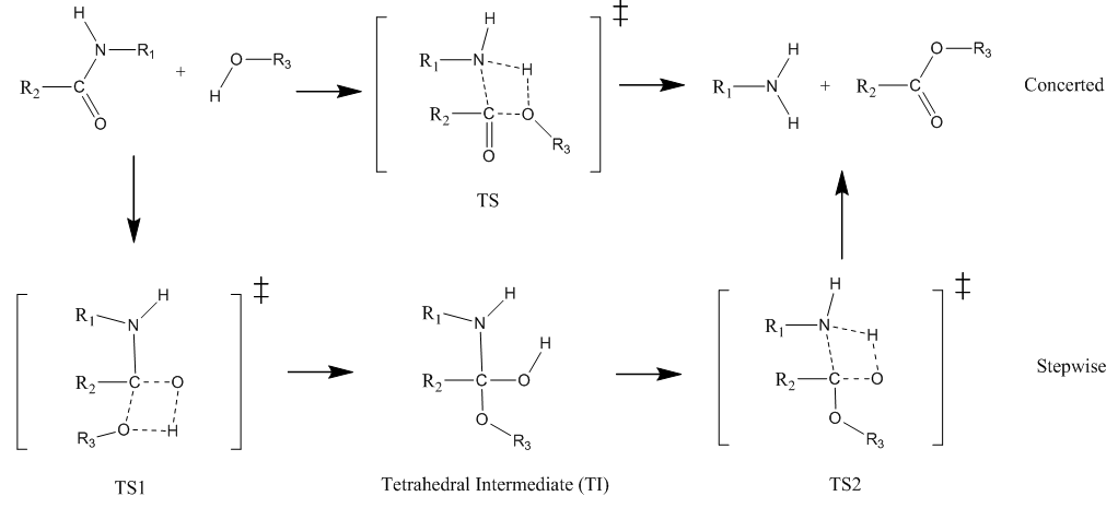
In this tutorial we shall investigate Potential Energy Surface of different reaction mechanisms of the peptide bond hydrolysis. Two main reaction mechanisms were proposed in the literature, Concerted and Stepwise:
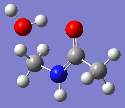
Our model system:
For the purpose of this tutorial it's easier to start from the stepwise mechanism.
The easiest way to start exploration of the Potential Energy Surface of a stepwise mechanism is to use a Tetrahedral Intermediate (TI) as a starting point. We shall pull Hydrogen from the OH group either to Oxygen or Nitrogen atom. Let's start from pulling the Hydrogen atom to other Oxygen:
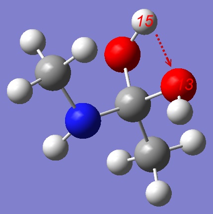
Gaussian input file is below:
# opt=(modredundant,maxcycles=250) rhf/3-21g Stepwise mechanism: pulling H towards other Oxygen 0 1 C -0.40953200 0.00511200 0.00217700 O -0.36936600 0.80863700 1.17619400 N 0.75806800 -0.81237200 -0.16394000 H 0.69402900 -1.69363600 0.30983300 C -1.66100300 -0.85199800 0.04995500 H -2.52312200 -0.20155100 0.04700900 H -1.69730600 -1.50949100 -0.80858500 H -1.66816900 -1.43878600 0.95853300 C 2.04838400 -0.13543700 0.03978000 H 2.18681200 0.19741800 1.06216300 H 2.84841400 -0.81076000 -0.23211300 H 2.09170400 0.72585800 -0.61244900 O -0.46144200 0.94949700 -1.07008800 H -0.20647400 0.51383300 -1.89310400 H -0.25299200 1.73259000 0.91598200 B 15 13 S 12 -0.100000 |
where a line "B 15 13 S 12 -0.100000" is a part of a modreduntant input section which is described in details in other tutorial. You can notice that we use option maxcycles=250 which sets the maximum number of optimization steps to 250 since the default number of optimization steps sometimes could be not enough (The default is the maximum of 20 and twice the number of redundant internal coordinates in use (for the default procedure) or twice the number of variables to be optimized (for other procedures).
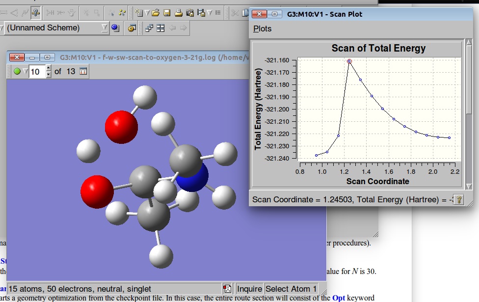
Below are results of the PES. We shall select a geometry corresponding to the Saddle point and use it as a starting point for the TS optimization:
Here is input file for Gaussian requesting for the TS optimization:
# opt=(calcall,tight,ts,maxcycles=250) rhf/3-21g TS1 0 1 C -0.38053300 0.10698400 -0.05899600 O -0.29500300 -0.80134000 -1.13362600 N 0.80734500 0.72933500 0.33129800 H 0.79423300 1.72357600 0.41225100 C -1.58104000 1.02202500 -0.08060200 H -2.46145400 0.42541600 -0.26053200 H -1.68495800 1.54991400 0.85929600 H -1.47006500 1.73627900 -0.88621600 C 2.08059500 0.10816200 -0.04125300 H 2.22136800 0.07061900 -1.11344400 H 2.88525300 0.67006400 0.41385000 H 2.11381700 -0.90318500 0.33994100 O -0.67948100 -1.10197800 0.82838300 H -0.48094400 -1.06114900 1.77365700 H -0.48692500 -1.51337100 -0.33083400 |
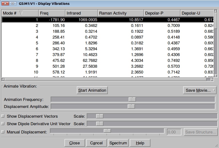
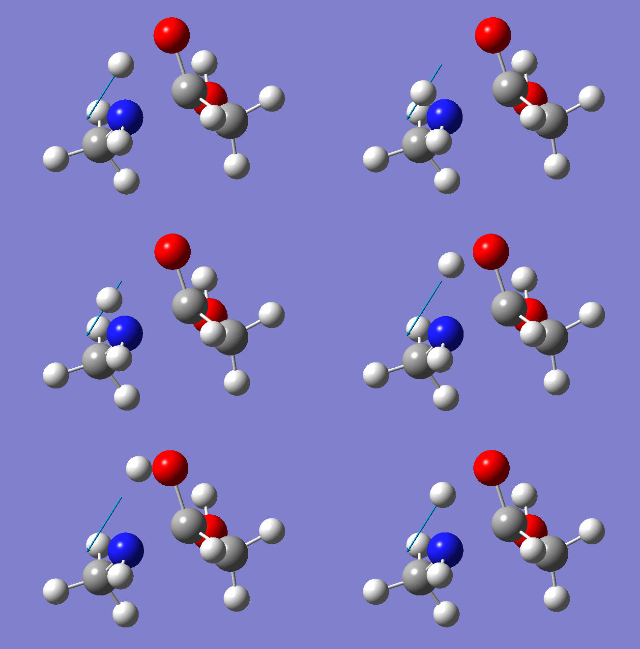
Here is the resulted output file and frequencies information:
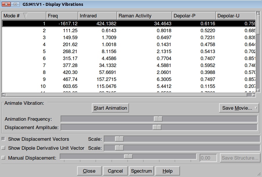
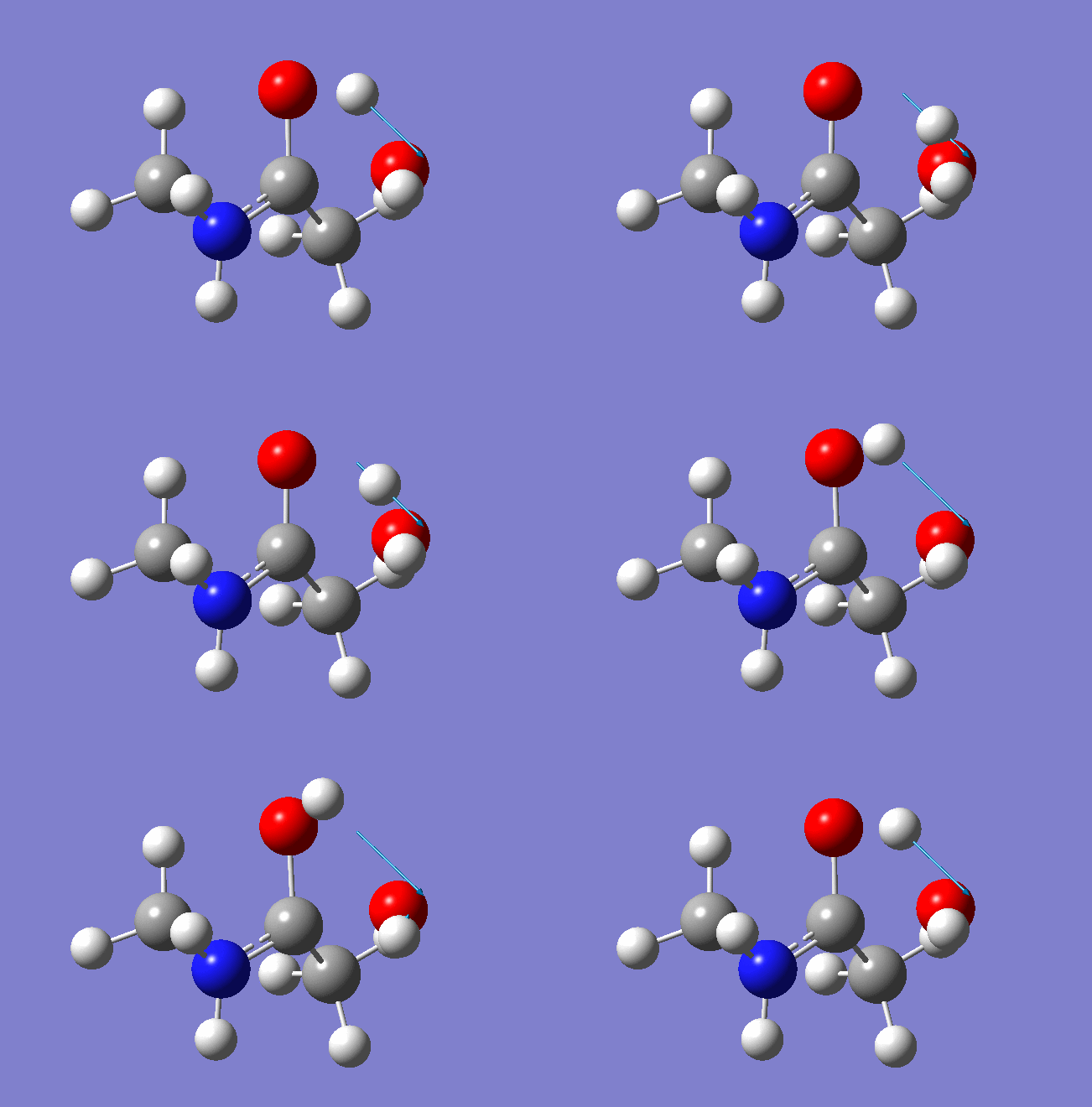
Now we shall do the same for pulling the Hydrogen atom to the Nitrogen:
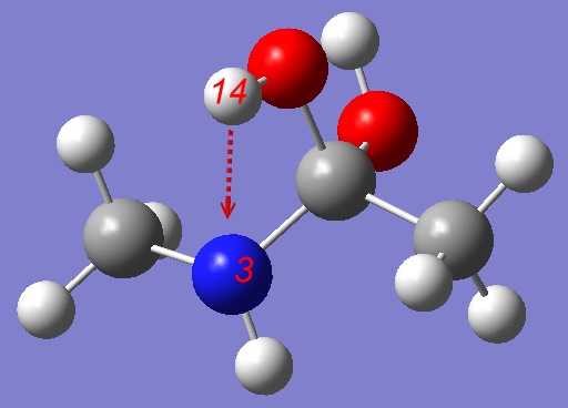
Here is Gaussian input file:
# opt=(modredundant,maxcycles=250) rhf/3-21g Stepwise mechanism: pulling H towards Nitrogen 0 1 C -0.40953200 0.00511200 0.00217700 O -0.36936600 0.80863700 1.17619400 N 0.75806800 -0.81237200 -0.16394000 H 0.69402900 -1.69363600 0.30983300 C -1.66100300 -0.85199800 0.04995500 H -2.52312200 -0.20155100 0.04700900 H -1.69730600 -1.50949100 -0.80858500 H -1.66816900 -1.43878600 0.95853300 C 2.04838400 -0.13543700 0.03978000 H 2.18681200 0.19741800 1.06216300 H 2.84841400 -0.81076000 -0.23211300 H 2.09170400 0.72585800 -0.61244900 O -0.46144200 0.94949700 -1.07008800 H -0.20647400 0.51383300 -1.89310400 H -0.25299200 1.73259000 0.91598200 B 3 14 S 15 -0.100000 |
The resulted output file and PES:
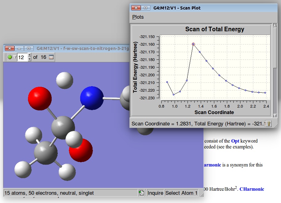
A structure corresponding to the Saddle Point was used for further TS optimization:
# opt=(calcall,tight,ts,maxcycles=250) rhf/3-21g TS2 0 1 C -0.51963800 -0.06997800 0.04591800 O -0.27084200 -1.31801700 -0.54695100 N 0.80040600 0.72017700 0.20920500 H 0.72470200 1.67232900 -0.11392100 C -1.55589300 0.68710400 -0.74640600 H -2.49021900 0.14581900 -0.69044600 H -1.70073400 1.66966900 -0.31809600 H -1.26017500 0.76746700 -1.78388000 C 2.03754600 0.07534900 -0.29137400 H 1.97429200 -0.13480000 -1.34962600 H 2.87491500 0.72983100 -0.09329400 H 2.18587100 -0.85309600 0.23605200 O -0.70071200 -0.14063000 1.43087800 H 0.31396100 0.45156900 1.36573800 H -0.22511300 -1.97569800 0.16279800 |
And here is the resulted output file and and frequencies information:
